Marco Bernasocchi, who is working on porting QGIS to Android at GSoC 2011, reports on a successful cross-compilation of QGIS using the Android NDK r5c.
This was preceded by work on porting all the libraries needed to build QGIS (GDAL, GEOS, Proj, etc). Porting SpatiaLite and optimising the interface for tablets are next on the list.
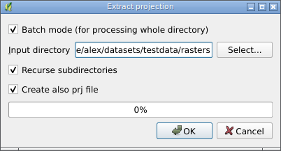
It is no secret that one of the most common raster formats, TIFF, is able to store georeferencing information within the file, turning it into a GeoTIFF. Everything would be fine if it weren’t for one nuance: the vast majority of graphic editors suffer from “star fever”, believing that unrecognised tags have no place in the file and happily removing this valuable information when saving the file.
This feature of graphic editors is often used to “reset” georeferencing (for example, if the image is incorrectly georeferenced and needs to be georeferenced from scratch). A natural question arises: what to do if you need to edit the image in a graphics editor but do not want to lose the georeferencing? The answer is not original, it is necessary to save it in an external file (the so-called world file).
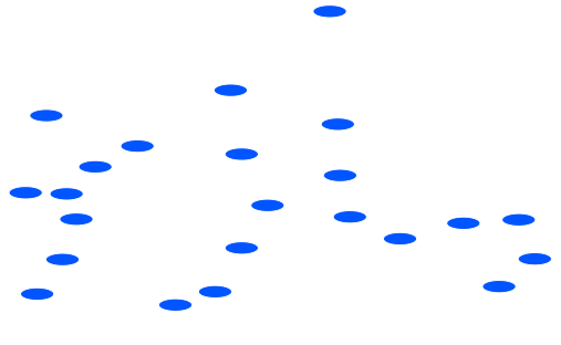
Marco Hugentobler has added a new marker type called “Ellipse” to QGIS. It looks like this
Point layer renderer using Ellipse marker
You can use this type of marker to create not only ellipses but also other shapes such as rectangles, triangles or crosses. Both the height and width of the marker can be changed; all basic parameters (fill colour, outline colour and thickness, rotation) are available, and most properties can be data-defined.
In the future, the Ellipse marker will be merged with the Simple marker.
QGIS Browser is now not only available as a standalone application but also integrated into QGIS. Martin has added a dockable Browser panel showing a directory tree and registered WMS connections. Double-clicking on a layer in the Browser panel adds it to QGIS.
And Pirmin Calberer has managed to get his Globe plugin into the QGIS core. More information about the plugin can be found here.
The initiative by kCube Consulting that they started last December failed miserably. The idea was that a full-time developer from this company would work on QGIS for half a year, and after discussion, the main focus of the work was determined — bug fixing. This may not be very interesting, but it is certainly useful.
Six months have passed… Nobody has seen the promised monthly reports. A search of the bugtracker reveals only 6 (six!) issues where our hero has “done” anything. Of these 6 bugs, only 2 (two, really?!) are actually closed, and one patch has been almost completely reworked by one of the core developers.
There is nothing to add other than the words from the post title.
After several delays and release postponements, QGIS 1.7 “Wrocław” has finally been released.
There are many reasons for the delays, but there are two main ones. The first is that the developers decided to devote the last meeting to bug fixing, and the second is an update to the project’s infrastructure. The repository is now hosted on GitHub, which has led to a revision of the repository access policy. The old Trac bug tracker has also been replaced by Redmine.
This release is notable not only because the release date has been pushed back several times but also because it is the last release in the 1.x series. (at least that is the plan). The next release will be QGIS 2.0, which is expected to have many groundbreaking changes: API updates, a final transition to a new symbology, and more. A point release of QGIS 1.7.x with bug fixes but no new features will be prepared from time to time. Closer to the release of QGIS 2.0, an interim release of 1.9.x is planned for a limited number of users.
Now about QGIS 1.7.0. This release contains over 300 fixes and many improvements. You can read the detailed description of the changes in the official announcement, but I will limit myself to a short list:
Marco Hugentobler has implemented the ability to embed layers and groups from other QGIS projects into a current project (available in both QGIS and QGIS MapServer). This can help eliminate the extra work of “laying out” data in a TOC when the same data is used in multiple projects. Simply go to the “Layer → Embed layers and groups” menu, select the source project, and select the desired layers/groups.
Embedding does not involve copying data but using links that can be either absolute or relative (depending on the project settings). Accordingly, any changes made in the source project will be reflected in the target project.
If you need “real” embedding, the ImportLayersFromProject plugin (by Barry Rowlingson) written the day before comes to the rescue. The plugin also analyses the source project and allows you to transfer a layer completely from one project to another. This eliminates the dependency on the source project, which can be modified or even deleted without losing the data embedded in the target project.
Often, novice QGIS users who have downloaded satellite images from Earth Explorer or other sources ask themselves: “What do I do with these files, and why do I see a black rectangle or a black and white image instead of a nice color image?” The thing is that satellite images are usually distributed as separate files, each of which corresponds to a specific radiation range (channel). To get a beautiful and informative image, these channels (often called bands) should be combined, and then, depending on the task, we need to choose the right band combination.
In this post I will show you how to do this in QGIS. I will assume that QGIS is already installed and that you already have a set of rasters that make up a multi-band image, such as a Landsat scene.