Hydrology analysis with TauDEM and SEXTANTE
15.12.2012 14:11 · GIS · qgis, processing, howto
TauDEM (Terrain Analysis Using Digital Elevation Models) is a set of Digital Elevation Model (DEM) tools for extracting and analysing hydrological information from the topography represented by a DEM. It was developed at Utah State University (USU) for hydrological analysis of digital elevation models and watershed delineation.
TauDEM has recently been integrated into QGIS as a SEXTANTE provider. This makes it possible to run TauDEM tools directly from QGIS, easily perform complex analysis workflows, and view the generated results.
In this post, I will show how to perform some hydrological analysis tasks in QGIS using TauDEM, namely how to delineate watersheds and extract stream networks.
Note
Please note that TauDEM is distributed as a set of standalone command line tools for Windows and as source code for other systems. SEXTANTE only contains the interface description, so you need to install TauDEM 5.0.6 and configure SEXTANTE properly.Let’s start.
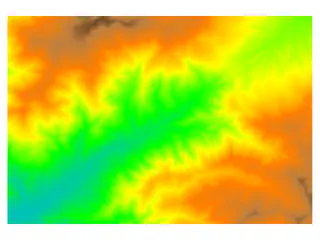
First, load the DEM into QGIS and adjust the symbology.
TauDEM extracts hydrologically useful information from raw digital elevation model data. The main idea is based on the concept that the hydrological flow field is represented by the flow from each raster cell to one or more of its neighbours. For this to work, the topography should contain no pits, defined as one or more raster cells completely surrounded by cells with higher elevation. Pit removal should be the first step in the hydrological analysis. TauDEM uses a fill process to do this, raising the elevation of pits until they drain out. A DEM with pits removed is called hydrologically correct and can be used to calculate flow directions for each raster cell.
So the first tool to run is “Pit Remove”. It has a single input called “Elevation Grid” where we should select our DEM and then run the algorithm.
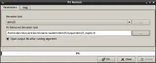
The output DEM is the same as the input DEM because our input file has no pits. If you are absolutely sure that your input file has no pits, this step can be skipped, otherwise it is safer to run “Pit Remove” to ensure that further analysis will be correct.
The next algorithm to run is “D8 Flow Directions”.
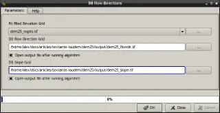
This tool takes as input the hydrologically correct elevation grid (which we created in the previous step) and outputs the D8 flow direction and slope for each grid cell. The resulting D8 flow direction grid is shown below.
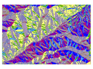
D8 is the simplest flow direction model. It uses an encoding of the direction of steepest descent from each grid cell using the numbers 1 to 8, to represent each one of the cells around a given cell.
Note
All TauDEM algorithms have built-in help, so you can always read a description of the algorithm, its inputs, and the results it produces.The next tool to run is “D8 Contributing Area”. It counts the number of grid cells draining through (out of) each grid cell based on the D8 flow directions.
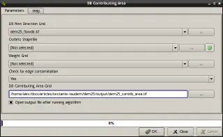
There are optional inputs in this algorithm (outlets and an input weight grid) which we will leave empty for now. These inputs are described in the algorithm help and allow us to restrict calculation to the specific area upstream of the designated outlet and to accumulate an input weight field, rather than just counting contributing area as a number of grid cells. There is also an option called “Check for edge contamination’ (set to “Yes” by default).
The layer produced by this algorithm looks like this
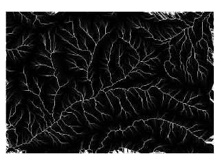
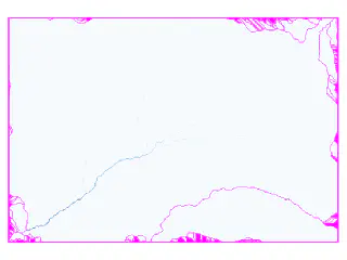
A logarithmic scale is better suited to the particular distribution of values in this layer. In the image below, the same grid is rendered using a logarithmic scale, and pink is used to show the NODATA values to illustrate edge contamination.
In this post I used the D8 flow model, which represents the flow from each grid cell to a neighbour. TauDEM also provides the D∞ (D-infinity) flow model, which calculates the steepest outwards flow direction using triangular facets centred on each grid cell and distributes the flow between neighbouring grid cells based on the flow direction angles.
With flow directions and slope grids, we can delineate and analyse stream network and watersheds. The simplest method of delineating stream network uses a threshold on contributing area.
First, we need to define streams using the “Stream Definition By Threshold” algorithm.
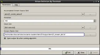
This tool defines a stream grid by applying a threshold to the input. In our case, the input is a D8 contributing area grid, and a threshold of 100 grid cells has been used.
The result represents the stream network as a binary grid (but not yet logically connected as a network shapefile).
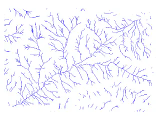
The next step is to define the outlet point. This can be done by creating a point shapefile and adding the outlet point to it. Press the “New Shapefile Layer” button in the main QGIS window to open the following dialogue,
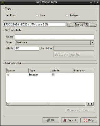
Select “Point” as the geometry type and select the same CRS as the DEM. TauDEM needs this because it doesn’t do any CRS transformations. Press “OK” and save the new file to a location of your choice. A new vector layer will be added to the QGIS canvas. Select it and start editing. Zoom to a likely location for an outlet and create a new point feature, then save edits and turn the editing mode off.
It is not necessary for the outlet to be located exactly where there will be a stream, as TauDEM has a tool for moving outlets to streams that we will use. Alternatively, if the outlet location is available from another source (e.g., stream gauge location information), it can be created from that information.
Here is the outlet we created manually
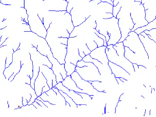
As you can see, it is outside the stream. So we use the “Move Outlets To Streams” tool to put the outlet in the right place.
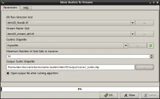
Warning
TauDEM creates a new shapefile in the same CRS as the input file, but it doesn’t create a.prj file. You need to manually define the projection for the output file so that it is displayed in the correct place. This can be done from the layer context menu using the “Set Layer CRS” item.Here is our original outlet (red) and the correct one (green). Note how the outlet has been moved to match the stream.
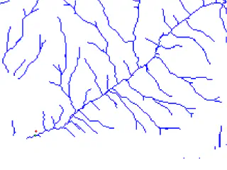
With the outlet positioned exactly on the stream, the stream network upstream of the outlet can be delineated.
We need to run the ‘D8 Contributing Area’ algorithm again, but this time specify an outlet shapefile to evaluate the contributing area and effectively identify the watershed upstream of the outlet point (or points for multiple outlets).
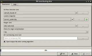
The result is the contributing area only for the watershed upstream of the outlet.
The next step is to use the “Stream Definition By Threshold” algorithm to define streams using a given contributing area threshold. I use a threshold of 200 grid cells.
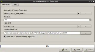
The result is a grid with stream network upstream of the outlet
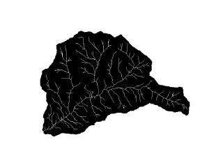
This network is still represented as a raster. The “Stream Reach and Watershed” algorithm is used to convert it to a vector network in shapefile format.
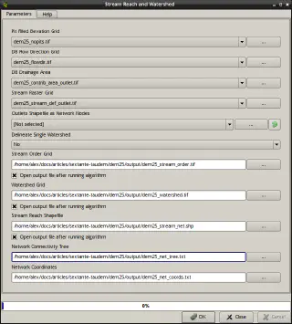
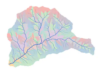
This algorithm produces many outputs, including a watershed grid and stream network shapefile, and some text files with additional information. Here I have visualised the watershed grid and stream network shapefile.
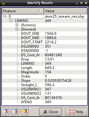
The attributes of a stream network link contain useful information such as downstream and upstream connectivity, stream order, length, slope, drainage area, etc. (detailed explanations of the fields are available in the tool help).
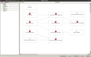
Instead of doing each step separately, we can create a model using SEXTANTE Modeler to run these algorithms together.
