Geoprocessing with SEXTANTE and QGIS
27.11.2012 17:55 · GIS · qgis, processing, howto
SEXTANTE is a powerful and flexible platform for performing geospatial analysis in QGIS. It provides access to its own geoprocessing functions as well as algorithms implemented in third-party applications, making analysis easier and more productive.
Initially written in Java and only available to gvSIG users, SEXTANTE has gradually extended its presence to other GIS. In 2012, a Python version was developed for use with QGIS. It immediately attracted a lot of interest from users and developers alike, and in September 2012 SEXTANTE was integrated into QGIS as a core plugin.
SEXTANTE in QGIS allows you to use the main features of well-known third-party GIS tools (SAGA GIS, GRASS GIS, TauDEM, OrfeoToolBox…) and algorithms implemented directly in SEXTANTE (fTools, MMQGISX…) via a unified interface.
It also offers a wide range of possibilities for automating data processing: combining repetitive steps of applying algorithms to data in a custom analysis model, writing and using Python scripts, batch processing mode. Advanced users can further increase their productivity by using SEXTANTE algorithms and the Python console together.
User interface
The SEXTANTE user interface consists of four main parts. Each of these allows you to run algorithms. The choice of method depends on your personal preferences, the data you are using, and your objectives. All interface elements (except the batch processing dialogue) are accessible from the “Analysis” menu.
Toolbox
The main GUI part of SEXTANTE is the SEXTANTE Toolbox, and this is probably what you will be using most of the time. All available algorithms are displayed here, organised into groups. From the Toolbox, you can run an algorithm in a single run or batch processing mode.
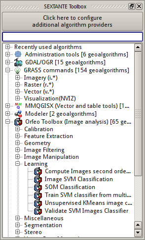
Each group in the toolbox represents a “provider”, i.e., a set of algorithms from the same source (e.g., a third-party application). Some of the algorithms belong to third-party applications (SAGA, OrfeoToolbox, TauDEM, GRASS…), while others are algorithms implemented directly in SEXTANTE (fTools, MMQGISX…). There are also two special groups, “Modeler” and “Scripts”, which are dedicated to user algorithms and allow users to create their own processing workflows.
At the top of the toolbox, there is an input field for filtering the list of available algorithms. Simply enter a word or phrase, and only those algorithms will remain in the list whose name or description contains the entered text.
Note
SEXTANTE only contains descriptions of the basic algorithms of SAGA, GRASS, OTB and other third-party applications. It should be noted that all these applications are not shipped with SEXTANTE. It is therefore not possible to run these algorithms, although they are shown in the Toolbox. In order to use algorithms from third-party applications, these applications must be downloaded and installed beforehand.It should also be noted that third-party algorithms are disabled by default. You can enable them in the configuration dialogue, which can be found in the “Analysis → SEXTANTE options and configuration” menu.
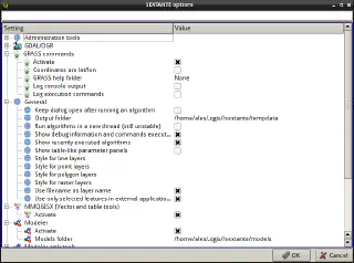
To enable algorithms, locate the application’s group in the list, expand it, and tick the “Activate” box.
Running an algorithm
Double-clicking on the algorithm name in the toolbox opens a parameter dialogue box where you can specify input data, algorithm settings, and the location of the generated outputs.
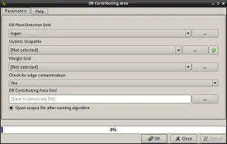
SEXTANTE algorithms support the following parameter types:
- raster layer — this can be either a layer loaded into QGIS or a file on disc
- vector layer — similar to a raster layer, can be selected from the list of loaded layers or by specifying a file on disc
Note
If the algorithm also has an attribute table field parameter, you can only select from the layers loaded in QGIS. - table — currently, only geometryless tables in DBF and CSV formats are supported
- selection — a drop-down list of predefined values from which you must choose one

Selection parameter in SEXTANTE - number — integer or floating point value. The button next to the input field opens a helper dialogue where you can enter an arithmetic expression and/or select some values extracted from the data loaded into the project (layer coverage, pixel size, etc.)
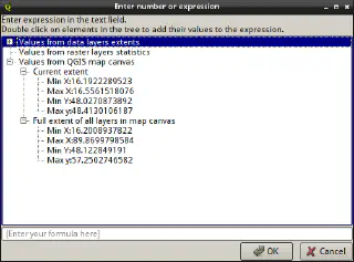
Helper dialogue for number parameter - range — a numerical interval defined by minimum and maximum values
- text — single- or multiline string value
- attribute (table field) — selected from the list of table or layer fields specified by another parameter
- CRS — either defined by EPSG code or selected from the list of available coordinate systems
- extent — defined by
xmin, xmax, ymin, ymaxvalues. Value can be entered manually or selected from the list of extents of loaded layers and the current map extent. It is also possible to draw the required area on the map
Extent selection menu 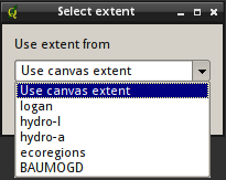
Extent selection dialogue 
Drawing extent on canvas - multiple input — multiple elements (e.g. layers) selected from the list of available elements
- fixed table — a small table edited by the user (e.g. recalculation settings for working with raster data)
Algorithms can produce the following outputs:
- raster layer
- vector layer
- table
- HTML (for text and/or graphics)
- file (a text file or any other file that does not fall into one of the above types)
In most cases, the output file format is determined by the file extension, and the list of supported file formats depends on the algorithm. If you do not specify an extension or specify an unsupported (including incorrect) extension, the result will be saved in the default format and the appropriate extension will be automatically appended to the filename.
If no filename is specified, the results are saved as temporary files and deleted when QGIS is closed.
In the settings (“Analysis → SEXTANTE options and configuration → General → Output folder”) you can specify a directory for the results. This path will be used if only the output file name is specified.
In addition to raster and vector layers, SEXTANTE can also handle results in HTML format. This format is typically used to display text and images (e.g. graphs). The HTML results are displayed at the end of processing in a special “SEXTANTE results viewer” window and are available throughout the working session.
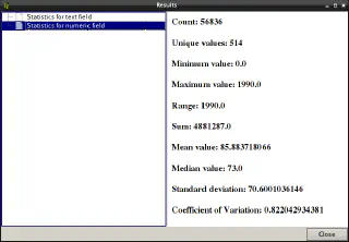
Some algorithms may produce files in formats not supported by QGIS (e.g. LiDAR survey files in LAS format). Such files will be saved to disk, but not added to the QGIS project. For all other file types (vector, raster and tabular) there is a checkbox to control whether the file should be loaded into the project. By default, all results are added to the project.
SEXTANTE does not yet support optional results, so if you uncheck “Open output file after running algorithm”, the output file will still be created (either as a temporary file or written to a user-defined path).
Graphical modeler
When an analysis is performed, it is rarely limited to a single operation/algorithm; more often, a series of sequential actions must be performed. That is, the analysis can be represented as a sequence of steps. The Graphical Modeler allows you to describe this sequence of actions once and then refer to it as a whole. This approach allows you to reduce the time required to process large amounts of data. It does not matter how many steps are required to achieve the result, the model is executed as a single algorithm.
You can open the Model Editor either from the “Analysis → SEXTANTE Modeler” menu or from the toolbar: in the “Modeler” group, there is a subgroup “Tools” with a single item called “Create new model”.
The Modeller window consists of two parts: on the left is a tab widget containing a list of possible model elements (input data and algorithms), and on the right is a canvas where the model is created.
The process of creating a model can be roughly divided into two stages:
- Defining model inputs. These inputs will be displayed in the algorithm dialogue box, and the user will be able to modify them before the model is run
- Defining workflow. Linking inputs to algorithms and defining the order in which algorithms are executed
Defining inputs
All available inputs are listed on the left side of the Modeller window, on the Inputs tab. The supported data types are:
- raster layer
- vector layer
- table
- table field
- string
- number
- boolean
Double-clicking on an input opens a parameter configuration dialogue box. The contents of the dialogue box vary depending on the type of parameter. Common to all parameters is the “Parameter name” field, where you must enter the name of the new input (this text will be used as the parameter label in the algorithm dialogue). The other fields vary depending on the type of parameter. For example, if a numeric input is selected, in addition to the name, you will need to specify a default value and a range of acceptable values.
You must also specify whether this input is required or optional.
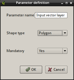
Once the fields have been filled in and the “OK” button has been clicked, a new block representing the input parameter is added to the modeler’s canvas.
Defining workflow
Once all the inputs have been added, we can begin to define the analysis workflow. The available algorithms are located on the Algorithms tab on the left side of the Modeler window. As in the case of the toolbox, the algorithms are grouped by provider, and there is also the option to filter the list.
To add an algorithm, double-click on its name in the list. This will open the algorithm settings dialogue box, which is similar to the one that opens when you run an algorithm from the Toolbox. However, there are some differences:
- raster and vector layers are still selected from the combo boxes. However, in this case, the combo boxes only contain layers defined as model inputs, as well as layers generated by other algorithms in the model
- strings and numbers can be either user-defined or selected from a list of values generated by other model algorithms
- table field. The list of table fields or layer fields is not known at the moment the model is created, as it depends on the layer that will be selected by the user. Therefore, in most cases, the field name must be entered manually. The only exception is when the model has a table field as an input, in which case it is possible to select from the drop-down list. The correctness of the field name entered is checked during model execution.
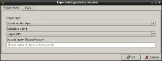
Once all the algorithm parameters have been defined, click “OK” and the algorithm block is added to the workspace. The algorithm block is linked to all other elements (model inputs and other algorithms) that provide inputs to this algorithm.
All model elements can be dragged and dropped around the canvas to rearrange them and make the model layout easier to understand. The relationships between elements are automatically updated.
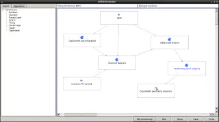
You can test the model at any time during its creation by pressing the “Run” button. However, to use the model from the Toolbox, you must save it and close the modeler window.
Saving model
Before you save a model, you must give it a name and specify which group within the toolbox it will be located in. These details are entered in the two fields above the modeler’s canvas.
The model is saved by pressing the “Save” button. By default, models are saved in the models subdirectory of the QGIS user directory, but this can be changed in the SEXTANTE settings (“Analysis → SEXTANTE Options and Configuration → Modeler → Models folder”).
When SEXANTE starts, it loads all models from this directory. All loaded models are displayed in the nested subgroups of the “Modeler” group in the toolbox and are also available in the Graphical Modeler window. This means that any model can be used as a regular algorithm when creating another, more complex model.
The model will not be loaded if at least one algorithm used in it is not found. This can happen if the required provider is disabled, making all its algorithms unavailable.
Editing model
As well as creating new models, SEXTANTE allows you to edit existing models. There are two ways to start editing a model:
- right click on the model in the toolbox to open the context menu and select ‘Edit model’
- open the Graphical Modeler, then click the “Open” button and select the model file on the disc
When editing a model, you can:
- change the links between inputs and algorithms
- add new blocks and/or delete existing blocks
- deactivate individual algorithms
When deleting an algorithm, remember that it can only be deleted if there are no other algorithms that depend on it. In other words, the results of the algorithm you are deleting must not be used anywhere else.
Sometimes it is necessary to exclude certain steps from the model without deleting them. In this case, the corresponding algorithm should be deactivated (open the context menu and select the corresponding item).
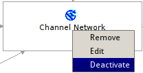
Deactivated algorithms are marked with the red label “[deactivated]”, and any algorithms that depend on them will be deactivated as well.
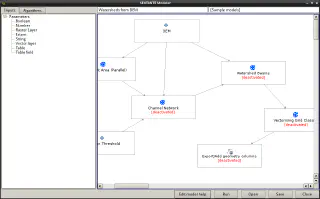
Activating a previously deactivated algorithm is very simple, just use the context menu again and select “Activate”.
Documenting models
It is considered good practice to document the models you create: add a description of the inputs, the actions taken and the result. This information will be useful to other users of the model.
Clicking the “Edit model help” button opens the model help editor dialogue.
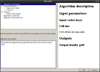
On the right is a simple HTML page generated from the model input and output labels. On the left, there are two fields: in the upper one, you select the element whose description you want to add, and in the lower one, you add the help text. The model help is automatically saved when you save the model in the same directory as the model itself.
Batch processing
All SEXTANTE algorithms, including models and scripts, can be run in batch mode. This means that they are not run once on a single dataset, but several times on different input datasets.
To run an algorithm in batch mode, select it in the Toolbox, right-click to open the context menu, and select “Execute as batch process”.
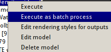
Starting a batch process is, in many ways, similar to running a single operation. The only difference is that the parameters are now set for each iteration. In this mode, the algorithm dialogue box looks like a table.
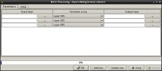
Each row of the table corresponds to a single iteration of the algorithm, and the cells contain the parameters.
By default, the table has three rows. If necessary, you can add or delete rows using the buttons at the bottom of the dialogue. Once the table size (number of rows in it) is set, you can start filling it with parameters.
Filling in parameters
Most parameters are set by either entering the required value in the box or selecting a value from the combobox.
Note that for batch processing, input layers (vector or raster) and tables must be selected from disk, not from the layers available in QGIS. Therefore, batch processing can be started at any time, even if the project is empty.
You can specify input file names either by entering the path to the file in the field, or by using the “…” button next to the corresponding field. In the latter case, a file selection dialogue with multiple selection support will open. If the parameter is a single file, the selected values are added to the table as separate rows (the table is automatically expanded to accommodate all the values). On the other hand, if the parameter accepts multiple values, all the selected files will be added to a single row.
In contrast to running the algorithm in normal mode, batch processing should save all results to files, the creation of temporary files is not allowed. The name of the output file can be specified either manually or using the file selection dialogue.
Automatic filling in of the parameters
Once the output file has been selected, another dialogue box opens, allowing you to fill in the rest of the output names automatically.
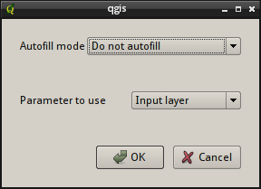
If “Do not autofill” is selected (default), SEXTANTE will simply insert the selected filename into the specified cell. If any other value is selected, all cells will be filled. In this case, filenames are generated based on the specified autofill criterion.
Both sequential numbers and values from other fields in the same row can be used for autocompletion. This approach greatly speeds up the filling of the batch processing parameter table.
History and log
Each time a SEXTANTE algorithm is executed, information about it is stored in the history. In addition to the name of the algorithm, all parameters and the date and time of execution are recorded. This makes it easy to retrieve and replay the sequence of operations.
You can view the history in the History window (“Analysis → SEXTANTE history and log”).
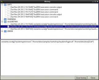
All events are displayed in chronological order, making it easy to find the data you need. The information is saved as a console command, even if the algorithm was run from the toolbox. This makes the History dialogue useful for learning SEXTANTE’s command line capabilities, as you can run an algorithm from the toolbox and then see in the History dialogue how to call it from the console.
As well as being able to view history items, you can also re-run any of them by double-clicking on the corresponding line in the history dialogue box.
The same window also contains other useful information: error messages, warnings, and additional information. If something is not working, you should check the “Errors” section.
Interaction with third-party algorithms is usually performed via the command line interface. Although the console is not shown to the user, all console output is redirected and stored in the “Info” section of the History dialogue. So, if something has gone wrong or there is any doubt about the correct execution of the tool, you will find all the messages generated by the algorithm in this section.
The “Warning” section usually contains various warnings about potential data problems (e.g., mismatched CRS). If you get an unexpected result, check if there are any messages in this section.
Using SEXTANTE in the Python console
The console allows power users to significantly increase their productivity and perform complex operations that are not possible with the SEXTANTE GUI.
SEXTANTE does not have a separate console. Instead, all SEXTANTE commands are available from the QGIS Python console. This means that we have all the features of the QGIS API and SEXTANTE at our disposal at the same time.
Code executed in the Python console, even if it does not call any SEXTANTE algorithms, can be converted into a new SEXTANTE algorithm, which can then be called from the toolbox or used in the Graphical modeler like any other algorithm.
Running algorithms from the console
The first thing we need to do to use SEXTANTE from the Python console is to import the SEXTANTE module:
import sextante
Now we can use SEXTANTE in the console, namely to run algorithms. To do this, we use the runalg() function. It takes the name of the algorithm as the first parameter, and then a variable set of additional parameters specific to the algorithm in question.
So the first thing we need to know is the name of the algorithm. Note that the algorithm name is not the same as the text displayed in the toolbox, but the unique internal name of the algorithm. You can find out the correct name by using the alglist() function. Just type in the console:
sextante.alglist()
and you will get something like this (the output is truncated):
D-Infinity Avalanche Runout-------------------------->taudem:d-infinityavalancherunout
D-Infinity Concentration Limited Accumulation-------->taudem:d-infinityconcentrationlimitedaccumulation
D-Infinity Contributing Area------------------------->taudem:d-infinitycontributingarea
D-Infinity Decaying Accumulation--------------------->taudem:d-infinitydecayingaccumulation
D-Infinity Distance Down----------------------------->taudem:d-infinitydistancedown
D-Infinity Distance Up------------------------------->taudem:d-infinitydistanceup
D-Infinity Flow Directions--------------------------->taudem:d-infinityflowdirections
D-Infinity Reverse Accumulation---------------------->taudem:d-infinityreverseaccumulation
D-Infinity Transport Limited Accumulation------------>taudem:d-infinitytransportlimitedaccumulation
D-Infinity Transport Limited Accumulation - 2-------->taudem:d-infinitytransportlimitedaccumulation-2
D-Infinity Upslope Dependence------------------------>taudem:d-infinityupslopedependence
D8 Contributing Area--------------------------------->taudem:d8contributingarea
The alglist() function prints information about all active algorithms in alphabetical order (algorithm name on the left, internal name on the right).
To avoid having to go through the whole list to find the algorithm you want, you can pass a filter string to the function, and only those algorithms with the given string in their description will be displayed. For example:
sextante.alglist("slope")
D-Infinity Upslope Dependence------------------------>taudem:d-infinityupslopedependence
D8 Extreme Upslope Value----------------------------->taudem:d8extremeupslopevalue
Slope Area Combination------------------------------->taudem:slopeareacombination
Slope Average Down----------------------------------->taudem:slopeaveragedown
Slope Over Area Ratio-------------------------------->taudem:slopeoverarearatio
Once we have the name of the algorithm, we should find out what parameters it needs to work. For this purpose, SEXTANTE provides the alghelp() function, which returns a list of input parameters and a list of output files generated by the algorithm. The only argument this function accepts is the internal name of the algorithm whose description we wish to obtain.
For example, here is help for the mmqgisx:creategrid algorithm:
sextante.alghelp("mmqgisx:creategrid")
ALGORITHM: Create Grid
   HSPACING <ParameterNumber>
   VSPACING <ParameterNumber>
   WIDTH <ParameterNumber>
   HEIGHT <ParameterNumber>
   CENTERX <ParameterNumber>
   CENTERY <ParameterNumber>
   GRIDTYPE <ParameterSelection>
   SAVENAME <OutputVector>
We can see that the algorithm is called “Create Grid” (this text is used in the toolbox), has 7 parameters (6 numbers and 1 is a selection), and generates a single output (a vector layer).
Now we have all the information we need to run the algorithm. As mentioned above, the algorithm is executed using the runalg() function. It has the following syntax:
sextante.runalg(name_of_the_algorithm, param1, param2, …, paramN, output1, output2, …, outputN)
The parameters and outputs depend on the algorithm, and should be specified in the same order as in the alghelp() output.
Depending on their type, parameter values are defined as follows:
- raster layer, vector layer or table — you can specify the name of the QGIS layer (if the layer is loaded in the project), the path to the file (if the layer is not loaded). Or you can pass a variable that is an instance of the corresponding QGIS class (e.g.
QgsVectorLayer). If the parameter is optional and will not be used — passNone - selection - the value is given as an integer index corresponding to the specific value. You can get the list of available values and their corresponding indices using the
algoptions()method. For example:Note that indexing starts from zero.sextante.algoptions("mmqgisx:creategrid") GRIDTYPE(Grid Type) 0 - Rectangle (line) 1 - Rectangle (polygon) 2 - Diamond (polygon) 3 - Hexagon (polygon) - multiple input — a list of values separated by semicolons. The elements can be either object names or file paths
- table field — name of an attribute table field, case-insensitive
- fixed table — a comma-separated list of values enclosed in quotation marks. Values are defined from left to right and from top to bottom. It is also possible to pass a two-dimensional array of an appropriate size
- CRS — an EPSG code of the desired CRS
- extent — xmin, xmax, ymin and ymax values separated by commas. For example
18.66629794, 18.70359794, 45.77670143,45.81170143
Number and boolean parameters can have default values. To use them, pass None in the corresponding position.
For algorithm results, the file path is specified, or None if it is to be saved to a temporary file. The file format is determined by the extension. If an invalid or unsupported extension is specified, the default format is used, and the appropriate extension is appended to the filename.
Unlike running the algorithm from the toolbox, the results are not automatically loaded into the project when processing is complete. You can load the results using either the QGIS API or by calling the SEXTANTE functions.
The runalg() function returns a dictionary, where the keys are the names of the outputs and the values are the paths to the corresponding files. You can add all the results to the canvas by passing this dictionary to the loadFromAlg() function. To load a single result, use the load() function.
Creating scripts
It is possible to create custom algorithms by writing the code in Python and adding a few lines of information specific to SEXTANTE. A simple script editor can be accessed from the SEXTANTE toolbox: group “Scripts”, subgroup “Tools”, item “Create new script”. In the editor dialogue that opens, you can type the script code. Scripts are saved script to the scripts subdirectory (default, can be changed in the preferences) of the sextante directory in the QGIS user’s home directory. Files should have `.py’ extension and the filename is used as the algorithm name in the toolbar (the extension is discarded and underscores are replaced with spaces).
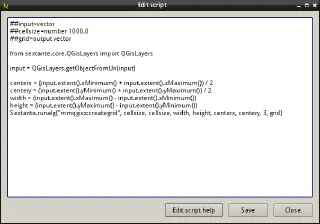
You can also create scripts in third-party text editors and save them in the SEXTANTE scripts directory.
Let’s look at a simple script to calculate the Topographic Wetness Index (TWI) from the DEM.
##[DEMO]=group
##dem=raster
##twi=output
ret_slope = sextante.runalg("saga:slopeaspectcurvature", dem, 0, None, None, None, None, None)
ret_area = sextante.runalg("saga:catchmentarea(mass-fluxmethod)", dem, 0, False, False, False, False, None, None, None, None, None)
sextante.runalg("saga:topographicwetnessindex(twi), ret_slope['SLOPE'], ret_area['AREA'], None, 1, 0, twi)
As you can see, there is nothing complicated about it. The scripts just execute three SAGA algorithms. If you read the previous section carefully, the code should be easy enough to understand. Now, we are most interested in the first three lines, which start with `##'.
The lines starting with ### are necessary for SEXTANTE to recognise the script, allow to execute it and use it in models like any other algorithm. The information in these lines has the following format
##[parameter_name]=[type_name] [additional_values]
Note that you must use underscores instead of spaces in the parameter name. However, the parameter or output type name can contain a space, e.g., `output vector'.
The first line is the name of the group to which our script will be added. Then come the parameters and outputs.
The following types of parameters can be used in scripts:
raster— raster layervector— vector layertable— tablenumber— integer or floating point number. The default value must be specified as the additional value. For example,##depth=number 2.4string— string, as with a numeric parameter, a default value must be specified in the additional values field. For example,##name=string NUMPOINTSboolean— boolean value. It is necessary to specify default value:TrueorFalse. For example,##verbose=boolean Truemultiple raster— list of raster layersmultiple vector— list of vector layersfield— attribute table field. It is necessary to specify the layer or table from which the field is taken. For example, if the script has the layer parameter defined asmylayer=vector, then the attribute field from the layermylayerwill be defined asmyfield=field mylayerfolder— directoryfile— a text file or any other file that is not one of the types listed above
The name of the parameter is used both as the label of the corresponding input field when the algorithm is run, and as a variable within the script to which the value entered by the user is assigned. When using the parameter name as a label, SEXTANTE replaces underscores with spaces. So if we call a parameter “Search_radius”, the user will see the label “Search radius” when running the algorithm from the toolbox.
Raster and vector layers, as well as tables, are passed to the script as strings containing the full path to the corresponding files on the disc. To get instances of the QgsVectorLayer or QgsRasterLayer classes from them, you can use the sextante.getObjectFromUri() method. Multiple objects are represented by a string containing file paths separated by semicolons.
Outputs generated by the script are described in the same way as inputs, using the following data types:
output rasteroutput vectoroutput tableoutput htmloutput fileoutput numberoutput string
A string containing the full path to the generated file is always written to the output variables. If the user has not specified a path to save the output, the corresponding variable will contain the path to a temporary file.
Note
SEXTANTE will attempt to load any results defined in the script header into the project upon successful script execution. Therefore, you should not use theload() and loadFromAlg() functions in the script, they are only needed when working in the console.When the algorithm performs time-consuming operations, it is useful to display the progress of the execution. For this purpose, SEXTANTE provides a progress' object. The setText()method allows you to display various information messages, and thesetPersentage()` method allows you to change the value of the progress bar.
Documenting scripts
As with models, a script can (and should) be accompanied by documentation. You can add a description to any script by opening it in the SEXTANTE script editor and clicking on the “Edit script help” button. The principle of creating help is the same as for models and needs no further explanation.
Example: Creating a density map using a hexagonal grid
Heatmaps are often used to visualise the density of points. But there are other approaches, one of which is to use a hexagonal grid. For this example, we will use data from the Viena Tree Cadastre.
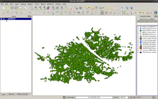
In general, the algorithm can be described as follows: we create a grid of hexagonal cells, count the number of points (trees) in each cell, and get a nice map.
The first thing we need to do is create a hexagonal grid. For this, we can use the “Create Grid” algorithm from the “MMQGISX” group. However, it has one drawback: it is necessary to manually specify the width and height of the grid, as well as the coordinates of its centre. This makes it very difficult to further automate the process. Therefore, we will write our own algorithm that creates a grid covering layer extent. Of course, we will not write it from scratch, but will reuse the MMQGISX algorithm that we already have.
Here’s the script:
# define script inputs and outputs

##input=vector
##cellsize=number 1000.0
##grid=output vector

# script body

from sextante.core.QGisLayers import QGisLayers

# input variable holds path to the vector layer. We need to create a QgsVectorLayer
# object from it to get layer extent
input = QGisLayers.getObjectFromUri(input)

# calculate grid parameters and run MMQGGISX algorithm
centerx = (input.extent().xMinimum() + input.extent().xMaximum()) / 2
centery = (input.extent().yMinimum() + input.extent().yMaximum()) / 2
width = (input.extent().xMaximum() - input.extent().xMinimum())
height = (input.extent().yMaximum() - input.extent().yMinimum())
sextante.runalg("mmqgisx:creategrid", cellsize, cellsize, width, height, centerx, centery, 3, grid)
Thus, our algorithm is essentially a “wrapper” over an existing algorithm, allowing us to generate a grid without having to specify its size.
Note
The script above is now part of the SEXTANTE plugin and is available as “Hex grid from layer bounds” in the “[Example scripts]” subgroup of the “Scripts” group.When you run the script, an algorithm dialogue box opens, just as when you run any other SEXTANTE algorithm.
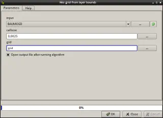
As an input layer we choose a point layer with trees, set the cell size to 0.0025 and on successful execution we get a hexagonal grid covering the input layer.
To count the number of points (trees) in each grid cell, let’s use the “Count points in poylygons” algorithm from the “fTools” group.
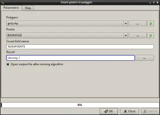
Here is the result, rendered with a graduated symbology, is shown below
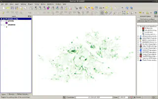
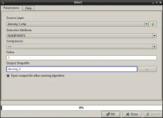
If you make the empty cells transparent, you will see that there are quite a lot of them. It would be nice to remove them to reduce the layer size. The “Select” algorithm from “MMQGISX” is perfect for this task. It will give us a new layer containing only cells with at least one point.
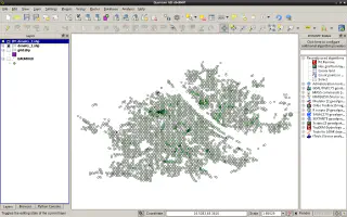
A slightly different symbology is deliberately used here (the cell borders are black) to show how the number of cells decreased after the empty cells were removed.
All these actions can be combined into a model and then performed in a single step. All you will need to do is select the input layer and the desired cell size.
Let’s open the model editor and define the model name and the group in which it will be saved. Then start adding inputs:
- vector layer. Let’s use “Input vector layer” as the label and set the layer type to “Points” as we will only be creating the density map for point layers
- number (grid cell size). The “Cell size” label should be quite informative, we will use
1000as the default value
The inputs are there, so we can start composing the algorithm. Let’s switch to the Algorithms tab and start adding algorithms in the order we ran them earlier:
- first, add the “Hex grid from layer bounds” algorithm we created. It has two inputs: a vector layer (select the layer input we added earlier from the combo box) and a numeric value (also select an input from the list). Note that we don’t write anything in the “grid” field, because the grid created in this step is not the final result, and we don’t need it
- now, find the “Count points in polygons” algorithm and add it. As a polygon layer we select the result generated by the “Hex grid from layer bounds” algorithm (named “grid from algorithm 0 (Hex grid from layer bounds)”) and as a point layer - the input vector layer. The name of the field with the number of points can be left unchanged or edited, let’s use the default value. We will also leave the “Result” field empty
- Add the last algorithm — “Select” from “MMQGISX”. As an input layer, we select the output of the “Count points in polygon” algorithm (“Result from algorithm 1 (Count points in polygon)”). As field names are not available at model creation time, we have to type the field name (
NUMPOINTS) ourselves. As a filter condition, we use≥1. And as this is our final result, we need to enter the name (label) of the output file, for example, “Output density grid”.
All that’s left is to arrange the blocks so that the model is easy to read, and then save it.
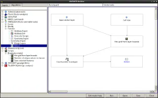
As you can see, the algorithm we have created can be used in the model. Moreover, the model itself can be used as a building block in another model, and the script created earlier can be used as part of a more complex script.
When you run the model, you will see the same dialogue just as when you run any other SEXTANTE algorithm.
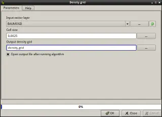
Note the labels of the input fields, they use the text we entered when defining the model inputs.
As you can see, by creating a model, we have achieved the same result as running several algorithms one after the other.